

Frequentist vs. Bayesian is an ongoing debate in the scientific research community. Which is best? Or can we even compare them?
Statistical inference is the process of making judgments about the parameters of a population using data drawn from it. Frequentist inference assumes events are based on frequencies, while Bayesian inference draws on prior knowledge.
This article takes a closer look at what each approach means and helps you figure out which to adopt for your analysis.
What you’ll learn in this post
• What frequentist statistics are and what Bayesian statistics are.
• The pros and cons of frequentist and Bayesian approaches for research data analysis.
• Why approach like the p-value may not give solid-enough evidence to support or refute your hypothesis.
• If there’s a reason to be strictly frequentist or strictly Bayesian in your data analysis.
• How you get get expert guidance on all aspects of your statistical methodology and results.
What are frequentist statistics?
A brief history
If you’re used to working with p-values and confidence intervals, or doing significance testing, then you’re using frequentist statistics. And that puts you in the majority.
Frequentist statistics were developed by mathematicians and statisticians Ronald Fisher, Jerzy Neyman, and Egon Pearson in the early 1900s. Fisher is known for developing the analyses of variance (ANOVA) in 1919 to better analyze the results of agricultural experiments.
Neyman and Pearson then created statistical hypothesis testing in 1933. Up until then, people were used to working with probabilities – concepts that gave rise to the field of modern statistics and hypothesis testing.
These concepts are central to frequentist statistics and have become the standard across most disciplines today. They’re also the main type of statistics taught in introductory statistics courses.
The frequentist view
Frequentist statistics are a type of statistical inference that tests whether an event (such as your hypothesis) occurs. Frequentists treat probabilities as equivalent to “frequencies” – the number of times something happens. These can be illustrated in a frequency graph, such as a pie chart or histogram, like this very basic one:

Frequentist statistics view probability as depending on the outcome of the experiment if you repeat it infinitely. So, if you flip a coin infinite times and get heads half the time, then the probability of getting heads (or tails by inference) is 50%.
However, in practice, this is done with a stopping criterion. This means that the coin toss will only be performed, for example, 2,000 times or until you get 200 heads. In real life, researchers don’t always repeat their study this number of times but will repeat it depending on the number of times necessary or appropriate for their field.
In frequentist reasoning, the parameters (e.g., the mean) that you try to estimate from your population are assumed to be fixed. You assume there’s a single true parameter that you’ll try to estimate, and the parameters are not modeled as a probability distribution.
Then, the random data points the experiment obtains are used to estimate the population parameter. Using this estimate, you can make probability computations regarding the data.
For example, if the height of a certain population is the parameter you try to estimate, you may hypothesize that the average height is 170 cm. This 170 cm is then taken as the true value. Then, you obtain data points (e.g., the heights of 75 different people in the population). You then use these data points to perform statistical tests.
What are the main tests frequentists use?
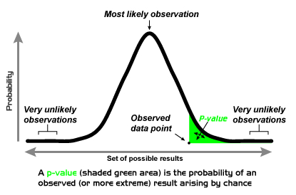
One of the main computations in frequentist statistics is the p-value. The p-value is a statistical measurement used to validate your hypotheses. The p-value represents the probability of getting a result as extreme or more extreme than the one you got if you repeated the study again, assuming the null hypothesis is true.
The way you compute a p-value depends on the tests you use for your study, such as a t-test or ANOVA. Each test has an underlying probability distribution. The p-value is calculated based on those underlying distributions.
The p-value will vary depending on the underlying distribution. For instance, if you performed a chi-square test, the p-value will be calculated based on the chi-square distribution and will be different from the p-value obtained from a t-distribution. But the interpretation of the p-value as a way to validate your hypothesis remains the same.
In practice, a significance level is specified in advance and which states how small the p-value needs to be to reject the null hypothesis. This significance level can vary depending on the discipline or journal. The standard significance level for the p-value is typically set at p<0.05 (i.e., the result occurs less than 5% of the time if the null hypothesis is true) across many research domains. However, some journals demand greater significance, and will only accept publications with the significance level set at p<0.01. (For practical ideas on the use of p-values, read this useful article by Sorkin and colleagues.)
If you obtain p=0.07, this means the result is likely enough under the null hypothesis that you wouldn’t reject that null hypothesis. If you get p=0.02, these results would be too unlikely under the null hypothesis. Here, you’d reject the null hypothesis and adopt the alternate hypothesis. This process is known as significance testing.
For example, your null hypothesis is that exercise has no effect on memory. Your alternate hypothesis is that exercise leads to better memory. You conduct a study by asking one group of participants to learn a list of words and then exercise. You then ask another group to learn the same list of words but to not exercise. Both groups then perform a recognition task on the words they learned. I then compare the performance on the tasks and get a p=0.07. You thus adopt the null hypothesis, assuming morning exercise has no statistically significant effect on memory.
Importantly, the p-value only measures the likelihood of the results occurring under the null hypothesis. It doesn’t give any information on the alternate hypothesis. This means that you could have results that are unlikely under the null, but almost as unlikely under the alternate hypothesis that you accepted. And this, in turn, could lead to unfounded conclusions in your research. (p-hacking is one undesirable byproduct of this.)
In significance testing, you also get a confidence interval around the p-value. The frequentist confidence interval reflects how sure you are that if you repeat the experiment again, your result will fall in that range. The confidence interval can be set at any percentage you deem is good enough for confidence, but it’s typically set at 95% in most research disciplines. A confidence interval of 95% means if you repeat the study again, you’d get results within the interval 95% of the time.
For example, a study found that sleep deprivation in young adults leads to decreases in associative memory. Participants underwent one night of sleep deprivation and then performed memory tasks. The researchers found a statistically significant p-value of 0.004 for memory scores following sleep deprivation. This finding means there’s a 0.4% chance of this result happening if the null hypothesis is true. Therefore, the null hypothesis (i.e., that sleep has no effect on memory) is rejected and the authors assume sleep deprivation somehow affects memory.
FREE PDF MINI-GUIDE
Reading and Interpreting Data and Graphs
This brief guide offers expert tips to help speed up and sharpen your reading and interpretation of data and graphs.
Our favorite section is Dr Lane’s amazingly handy step-by-step process (“D-I-K-U-W-D-A-I”) for visualizing data!
Advantages and disadvantages of using frequentist statistics
Frequentist statistics’ main advantage is user-friendliness. They’re “easier” to use and interpret. This is why they’re standard across many disciplines. However, they only give you point estimates rather than probabilities and are dependent on the number of times the study is conducted. Also, the p-value obtained only gives you information on the null hypothesis.
Advantages of frequentist statistics
- You have a specific test for each type of data
- You don’t need to have any prior knowledge of the data
- The standard across most medical and research practices
- Easy to interpret
- Computationally easy to do
Disadvantages of frequentist statistics
- Rigid frameworks
- You only get a “yes” or “no” answer and a point-estimate to your questions
- Results of the experiment depend on the number of times It’s conducted
- Experimental design must be specified in advance
- The p-value is not informative for the alternate hypothesis, it only computes the likelihood of the null hypothesis
What are Bayesian statistics?
A brief history
The statistical rival to frequentism is the Bayesian approach to statistical inference. If you’re used to working with priors and posteriors, and use the phrase “It is what you believe it is,” then you’re probably a Bayesian.
Bayesian statistics were developed by Thomas Bayes, an 18th-century English statistician, philosopher, and minister. Bayes became interested in probability theory and wrote essays in the mid-1700s that created the mathematical groundwork for Bayesian statistics.
Much of Bayes’ work, however, received little attention until around 1950. During this time, the rise of computers made it easier to do Bayesian statistics using machines with higher computing power.
The Bayesian view: What is Bayes’ Theorem?
The Bayesian worldview is based on Bayes’ Theorem. This is a mathematical formula that considers the probability of an event based on prior knowledge of conditions related to that event. This formula tells you how your current belief should be updated with data to get your new beliefs. Bayes Theorem is calculated by:
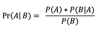
where P(A) is the probability of A occurring, P(B) is the probability of B occurring, P(A|B) is the probability of A given event B, P(B|A) is the probability of B given event A. In a Bayesian setting, A corresponds to the parameters and B to the data.
Pr(A|B) in the above equation is called the posterior, or the probability of the parameters given the data. P(A) is the prior, which is the probability assigned to the parameters before the experiment. P(B|A) is the likelihood, which is the probability of the data given the parameters. Finally, P(B) is the evidence, or the probability of the data, and is also the part that can make Bayesian approaches difficult to compute.
Unlike frequentists, Bayesians view probabilities as a measure of belief in the likelihood of an event happening. And they assume that parameters have a distribution instead of a fixed point, as in frequentist.
These beliefs may also get updated if new information (data) becomes available. The Bayesian approach calculates the probability that a hypothesis is true by updating prior opinions about the hypothesis as new data emerge.
This prior opinion is known as the prior probability before the study is conducted. Bayes Theorem then converts the prior into a posterior probability, which is the belief after the study has been conducted. This posterior is the probability of the parameter, given the results of the study.
For example, before conducting the coin-tossing experiment, you may believe the coin toss is fair, meaning it will follow a normal Gaussian distribution with a mean of 0. This is the prior distribution. Then, during the coin toss, you get heads 5 times out of 10 flips. The posterior distribution is then calculated based on the data acquired (5 heads out of 10) and the prior distribution.
The ability to incorporate our beliefs into hypotheses and to get a probability distribution over the parameters are the central tenets of the Bayesian approach. This is also one of the main reasons why some researchers are so strongly in favor of this approach. It’s something you can’t do with frequentism.
What are the main tests Bayesians use?
In Bayesian statistics, results are described in terms of the likelihood of one hypothesis over another. This is calculated by the Bayes factor (BF) shown below:
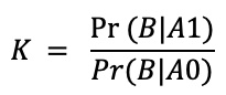
Where K is the Bayes Factor notation, Pr(B|A1) is the probability of the data given your alternate hypothesis, Pr(B|A0) is the probability of the data given the null hypothesis.
The BF can be set at any number that researchers believe is appropriate for the cutoff in their research. A BF of 20 is typically used to indicate evidence for a hypothesis and a BF of 1 is used to indicate no evidence. For instance, if your BF is 30, you have evidence for your hypothesis and if it’s 10, you have less evidence for the hypothesis.
With Bayes factors, we get a ratio between the null hypothesis vs. the alternate hypothesis. This allows researchers to get a strength of evidence of one hypothesis over the other. That’s also something you don’t have with the frequentist point-estimate approach.
In addition to the Bayes factor, Bayesian statistics also produce a credibility interval over the parameters. This is similar to the frequentist confidence interval, but it’s a range in which you’re 95% certain of your results.
For example, one study reviewed the effects of various drugs on depression and anxiety using a Bayesian approach. The researchers found that only half of the drugs obtained strong support for efficacy, indexed by BFs of over 20. Moreover, some drugs previously grouped as effective using significant p-values, obtained BF values of less than 1, meaning support for lack of efficacy.
In the above article, if one drug was classified as effective based on passing significance testing with p=0.002, we’d think that this anti-depressant was statistically proven to be effective. However, with a BF=1, we’d think that the evidence for the efficacy may not actually be that strong.
Thus, one of the Bayesian approach’s greatest advantages is that it allows us to acquire information on the strength of evidence for our results. We don’t get this information with the p-value point estimate. Such information is highly valuable in clinical research.
The 12P Method for Systematic Reviews
We’ve squeezed all the steps and stages of a typical systematic review onto one page.
You can print it out A4-sized and use it as a handy checklist, or A3-sized to post on your laboratory wall.
FREE PDF CHECKLIST
12P-SLR-Method-A3-print-v1.10-ENGAdvantages and disadvantages of using Bayesian statistics
The main advantage of Bayesian statistics is that they give a probability distribution of the hypotheses. They also allow the addition of new information to the hypotheses in the form of the posterior distribution.
However, creating the prior distribution can be tricky because there’s no predefined set of priors. This makes them seem arbitrary and it’s potentially not valid to assume something about the data that isn’t actually there.
Advantages of Bayesian statistics
- More intuitive
- Gives you a range between which you can be certain for or against your hypotheses rather than a point-estimate
- All information is contained within the data itself as opposed to unobserved frequencies
- Calculates the probability distribution of the hypotheses
Disadvantages of Bayesian statistics
- Setting the prior probabilities of the hypothesis can be different values because they’re subjective, thus making them appear arbitrary
- Bayesian analyses are complex and can require advanced statistical packages and software
- Require more advanced statistical knowledge
Summary of Frequentist vs. Bayesian Approaches
| Approach | What does it assume? | What does it ask? | What do you need? | What does it give? | Main advantages | Main drawbacks | When to use it |
| Frequentist | Parameters that you estimate are fixed and are a single point | Is the hypothesis true or false? | A stopping criterion
A predetermined experimental design |
A point estimate (p-value) | Simple and easy to use
Widely accepted Don’t need a prior |
Significance depends on the sample size
Only gives you a yes/no answer |
When you have a large amount of data |
| Bayesian | There’s a probability distribution around the parameters | What is the probability of the hypothesis given the data? | A prior
Any data set |
A probability for or against the hypothesis | You get strength of evidence Can update it with new information |
Priors can be subjective or arbitrary
Requires advanced statistics |
When have limited data
When you have priors When you have computing power |
Which should you choose? Or can you use both?
Now that we have some background on both frequentist and Bayesian approaches, you’re probably wondering which one is better to apply to your next analysis.
But there’s no right or wrong answer. You should choose the statistical approach based on the type of information and data you have.
Factors to consider before you choose
If you have certain beliefs or knowledge about your area of research, a Bayesian approach might be better, such as if you believe certain parameters to be true before conducting your experiment. If you have no prior beliefs about the data or you think the priors are not valid, then adopt a frequentist approach.
Bayesian approaches are also better if you have a small data set. For instance, if you have a dataset of only 10 data points, it will be difficult to get any statistical significance with a frequentist approach due to low power.
But you can always compute a BF.
This is because the prior distribution in Bayesian statistics can help even out extreme values.
If you have a lot of data from only one experimental study at one point in time, then a Frequentist approach could be more useful. This is because you can select the correct statistical test that matches the experimental design used. However, if you obtained your data over time or you plan to obtain new data, then a Bayesian approach is preferable because it lets you update it with new information.
You can also choose which approach to go with depending on how you want to deal with uncertainty. Frequentist statistics try to do away with uncertainty by providing point estimates, while Bayesian statistics preserve uncertainty by adjusting the priors with new information.
For instance, a p-value of 0.03 gives you a limited range of certainty, but a BF factor of 15 gives you a strength of evidence for or against your hypotheses. So if you want to convey uncertainty, go Bayesian.
It also depends on your computing power and statistical knowledge. Bayesian statistics can require more sophisticated statistical packages and computing power, while frequentist statistics can be easily applied in any computer program.

Can you use both?
Most studies usually have one type of approach that’s more appropriate depending on the size of their dataset, the design, and the models used.
For instance, if the model is too complex, you’ll typically have to use frequentist analyses and if you have a very small dataset, you’ll use Bayesian due to power issues. This approach is typically specified in advance, before beginning the experiment or data collection.
In cases where you can use both approaches, it’ll come down to if you want to incorporate a prior. If yes, then go Bayesian. If not, stay a frequentist.
It’s not very common to combine frequentist and Bayesian analyses in the same study because they’re based on different underlying assumptions. But sometimes it can be useful to use Bayesian approaches to re-analyze studies done with frequentist statistics. For instance, it could be valuable to re-analyze meta-analyses with a Bayesian approach
to determine the strength of evidence of certain variables using BFs.
Be careful when trying to use both approaches unless it’s well-justified. This can be seen as fishing for significance.
So which is better, Bayesian or frequentist? Both have their strengths and weakness and the ultimate decision should be made based on your data and assumptions. The good news is you don’t have to subscribe to one camp forever—you can always try out new statistical approaches.
Frequentist or Bayesian, a second look is always valuable
Whether or not you love statistics and take great joy in working your calculations, a second opinion or a helping hand can always make your work better. Edanz Statistical Analysis services put expert statisticians to work for you. No matter your technique, they can advise on your techniques and approach, help make your clinical data more robust, and give you an expert review of your results. Inquire with us for more details.